Shallow water gravity wave

This example is to demonstrate how to simulate shallow water gravity waves in a 2D domain enclosed by solid walls. The fluid is represented by a single homogeneous layer of which the progostic variables are

• u: velocity component in x direction

• v: velocity component in y direction

• \(\eta\): displacement of the interface hight, proportional to bottom pressure anomaly

The motion is governed by the following equations

• momentum equation along the x direction:

  \(\frac{\partial u}{\partial t} = -g\frac{\partial \eta}{\partial x}\)

• momentum equation along the y direction:

  \(\frac{\partial v}{\partial t} = -g\frac{\partial \eta}{\partial y}\)

• the continuity equation:

  \(\frac{\partial \eta}{\partial t} = -H\frac{\partial u}{\partial x} - H\frac{\partial v}{\partial y}\)

where the terms on the right-hand side of the momentum equations are the two components of the pressure gradient force (although is is actually the acceleration due to that force), and the two terms on the right side of the continuity equation are the change of the interface due to convergence of the flow along x and y direction.

Set the grid

the first step is to set up the computational domain. In this case, we want to solve the above equations on a rectangular domain that has a uniform grid spacing where the two spatial directions are always perpendicular to each other. Put more simply, we want to work on a cartesian grid. More precisely, we choose a representation of the prognostic variables such that they are defined on individual cartesian grids which are shifted to each other. This is called a staggered grid and for the problem at hand, the Arakawa C-grid is the best choice.

To create a set of cartesian grids staggered as a C-grid, we use the cartesian_c_grid factory method of the StaggeredGrid class.

import numpy as np
import matplotlib.pyplot as plt
from  multimodemodel import StaggeredGrid

nx, ny = 100, 100
dx, dy = 1., 1.

x = np.arange(0., dx * nx, dx)
y = np.arange(0., dy * ny, dy)

c_grid = StaggeredGrid.cartesian_c_grid(x=x, y=y)

OMP: Info #273: omp_set_nested routine deprecated, please use omp_set_max_active_levels instead.

The c_grid object provides all the necessary grid information for the sub-grids. E.g. the grid box size of the grid on which \(\eta\) is defined can be accessed like this

display(c_grid.eta.dx)

array([[1., 1., 1., ..., 1., 1., 1.],
       [1., 1., 1., ..., 1., 1., 1.],
       [1., 1., 1., ..., 1., 1., 1.],
       ...,
       [1., 1., 1., ..., 1., 1., 1.],
       [1., 1., 1., ..., 1., 1., 1.],
       [1., 1., 1., ..., 1., 1., 1.]])

Set the initial state

The next step is to define the initial state. We want to start from rest (\(u = v = 0\)) with an intial bump-like interface disturbance.

import matplotlib.pyplot as plt

x, y = c_grid.eta.x, c_grid.eta.y
eta = np.exp(
    -((x - x.mean()) ** 2 + (y - y.mean()) ** 2)
    / (x.max() // 5) ** 2
)

plt.pcolormesh(c_grid.eta.x, c_grid.eta.y, eta, shading='auto')
plt.axis('equal')
plt.colorbar()

<matplotlib.colorbar.Colorbar at 0x19c109a60>

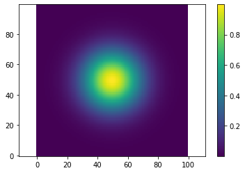
The numpy arrays needs to be turned into Variable objects which also know about the grid and time they are defined. For the time information, multimodemodel internally uses numpy.datetime64 objects. However, since we need to rely on the numeric representation of datetime, it is recommended to use the function multimodemodel.util.str_to_date function to create those dateimte64 objects. Finally the variables are joined into a state object which are used to express the current state or state changes of the system. Note that, for convenience, we can use None as data for variables that contain only zeros.

from multimodemodel import State, Variable
from multimodemodel.util import str_to_date

t0 = str_to_date("2001-01-01 00:00")

initial_state = State(
    u=Variable(None, c_grid.u, t0),
    v=Variable(None, c_grid.v, t0),
    eta=Variable(eta, c_grid.eta, t0)
)

Define the problem to solve

To solve the set of equations introduced initially, time stepping methods are applied. These methods need evaluations of all the right-hand sides of the governing equations. Hence, we define a function that is delivering exactly that. The function needs to take a State object as first argument and a parameter object (defining constants, etc.) as its second argument. More on the Parameter objects later.

from multimodemodel import (
    pressure_gradient_i,
    pressure_gradient_j,
    divergence_i,
    divergence_j,
    sum_states,
)

def non_rotating_swe(state, params):
    rhs = sum_states(
        (
            pressure_gradient_i(state, params),
            pressure_gradient_j(state, params),
            divergence_i(state, params),
            divergence_j(state, params)
        )
    )
    return rhs

Note that the different contributions, e.g. pressure_gradient_i, have the same signature as non_rotating_swe and return state increments. Examples for the structure of these functions can be found in kernel.py

Now we need to set some physical constants of the system, e.g. the depth of the fluid H. See the docstring of the Parameter class for more values to set, although not all are used in this example.

from multimodemodel import Parameter

params = Parameter(H=1.)

Solve the problem

Now we have all necessary ingredients set up to solve the problem. The only thing we need to do is to choose the time stepping scheme, the 3rd order Adams-Bashforth scheme here, the time step size step and the integration time time. The final state of the problem is obtained by calling the integrate function with all the required arguments.

from multimodemodel import integrate, adams_bashforth3

for next_state in integrate(
    initial_state, params, RHS=non_rotating_swe,
    scheme=adams_bashforth3, step=0.05, time=25.):
    pass

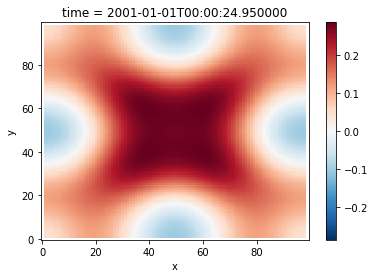
To visualize the output, we can use the handy as_dataarray property of the Variable class. It returns a copy of the data and grid information wrapped into a xarray.DataArray which offers among many other things a very usefull and feature rich plotting API.

next_state.eta.as_dataarray.plot(x='x', y='y');

Alternative API for solving the problem

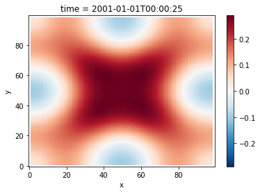
Instead of using the integrate generator, we can also make use of the Workflow class, that is orchestrating the workflow of integrating a set of PDEs over time. The workflow object needs an instance of the Solver class that provides the value at the next time step through its integrate method. We also need to wrap the initial state into a Domain object which keeps track of the parameters and the previous evaluations of the right-hand-side.

from multimodemodel import Domain, Solver, Workflow

domain = Domain(state=initial_state, parameter=params)

solver = Solver(rhs=non_rotating_swe, ts_schema=adams_bashforth3, step=0.05)

workflow = Workflow(domain=domain, solver=solver)

workflow.run(steps=500)

workflow.domain.state.eta.as_dataarray.plot(x='x', y='y')

<matplotlib.collections.QuadMesh at 0x19c31ccd0>

Although this approach seems more complicated than using the integrate generator, it allows to easily handle more complex workflow scenarios such as distriuting the computation accross a cluster of workers.